Exercise 4 Analysing some data with R
In this exercise we will use the R functions we have already used and the functions we have added to R to
analyse a small dataset. First we will start R and retrieve our functions:
load("tab2by2.r")
load("lregor.r")
And then retrieve and attach the sample dataset:
gudhiv <- read.table("gudhiv.dat", header = TRUE, na.strings = "X")
attach(gudhiv)
This data is from a cross-sectional study of 435 male patients who presented with sexually transmitted infections at an outpatient clinic in The Gambia between August 1988 and June 1990. Several studies have documented an association between genital ulcer disease (GUD) and HIV infection. A study of Gambian prostitutes documented an association between seropositivity for HIV-2 and antibodies against Treponema pallidum (a serological test for syphilis). Prostitutes are not the ideal population for such studies as they may have experienced multiple sexually transmitted infections and it is difficult to quantify the number of times they may have had sex with HIV-2 seropositive customers. A sample of males with sexually transmitted infections is easier to study as they have probably had fewer sexual partners than prostitutes and much less contact with sexually transmitted infection pathogens. In such a sample it is also easier to find subjects and collect data. The variables in the dataset are:
| MARRIED | Married (1=yes, 0=no) |
| GAMBIAN | Gambian Citizen (1=yes, 0=no) |
| GUD | History of GUD or syphilis (1=yes, 0=no) |
| UTIGC | History of urethral discharge (1=yes, 0=no) |
| CIR | Circumcised (1=yes, 0=no) |
| TRAVOUT | Travelled outside of Gambia and Senegal (1=yes, 0=no) |
| SEXPRO | Ever had sex with a prostitute (1=yes, 0=no) |
| INJ12M | Injection in previous 12 months (1=yes, 0=no) |
| PARTNERS | Sexual partners in previous 12 months (number) |
| HIV HIV-2 | positive serology (1=yes, 0=no) |
Data is available for all 435 patients enrolled in the study.
We will start our analysis by examining pairwise associations between the binary exposure variables and the
HIV variable using the tab2by2() function that we wrote earlier:
tab2by2(MARRIED, HIV)
tab2by2(GAMBIAN, HIV)
tab2by2(GUD, HIV)
tab2by2(UTIGC, HIV)
tab2by2(CIR, HIV)
tab2by2(TRAVOUT, HIV)
tab2by2(SEXPRO, HIV)
tab2by2(INJ12M, HIV)tab2by2(MARRIED, HIV)##
## outcome
## exposure 0 1
## 0 321 13
## 1 93 8
##
## Relative Risk : 1.043751
## 95% CI : 0.9818512 1.109554
##
## Sample Odds Ratio : 2.124069
## 95% CI : 0.8545749 5.279433
##
## MLE Odds Ratio : 2.119801
## 95% CI : 0.7380371 5.714354tab2by2(GAMBIAN, HIV)##
## outcome
## exposure 0 1
## 0 73 4
## 1 341 17
##
## Relative Risk : 0.9953155
## 95% CI : 0.9400068 1.053879
##
## Sample Odds Ratio : 0.909824
## 95% CI : 0.2974059 2.783333
##
## MLE Odds Ratio : 0.9100104
## 95% CI : 0.2853202 3.826485tab2by2(GUD, HIV)##
## outcome
## exposure 0 1
## 0 339 12
## 1 72 9
##
## Relative Risk : 1.086538
## 95% CI : 1.003531 1.176412
##
## Sample Odds Ratio : 3.53125
## 95% CI : 1.434372 8.693509
##
## MLE Odds Ratio : 3.517408
## 95% CI : 1.258556 9.491924tab2by2(UTIGC, HIV)##
## outcome
## exposure 0 1
## 0 261 12
## 1 151 9
##
## Relative Risk : 1.013027
## 95% CI : 0.9678841 1.060275
##
## Sample Odds Ratio : 1.296358
## 95% CI : 0.5338453 3.147997
##
## MLE Odds Ratio : 1.295532
## 95% CI : 0.4703496 3.438842tab2by2(CIR, HIV)##
## outcome
## exposure 0 1
## 0 10 3
## 1 392 17
##
## Relative Risk : 0.8025903
## 95% CI : 0.5955085 1.081682
##
## Sample Odds Ratio : 0.1445578
## 95% CI : 0.0364195 0.5737851
##
## MLE Odds Ratio : 0.1460183
## 95% CI : 0.03322189 0.899754tab2by2(TRAVOUT, HIV)##
## outcome
## exposure 0 1
## 0 152 2
## 1 256 19
##
## Relative Risk : 1.060268
## 95% CI : 1.02181 1.100173
##
## Sample Odds Ratio : 5.640625
## 95% CI : 1.295879 24.55218
##
## MLE Odds Ratio : 5.624226
## 95% CI : 1.32716 50.45859tab2by2(SEXPRO, HIV)##
## outcome
## exposure 0 1
## 0 268 13
## 1 143 8
##
## Relative Risk : 1.007093
## 95% CI : 0.9621259 1.054161
##
## Sample Odds Ratio : 1.153308
## 95% CI : 0.4671083 2.847562
##
## MLE Odds Ratio : 1.152912
## 95% CI : 0.4042323 3.083152tab2by2(INJ12M, HIV)##
## outcome
## exposure 0 1
## 0 146 7
## 1 268 14
##
## Relative Risk : 1.004097
## 95% CI : 0.9610996 1.049018
##
## Sample Odds Ratio : 1.089552
## 95% CI : 0.4301305 2.759916
##
## MLE Odds Ratio : 1.089351
## 95% CI : 0.4006202 3.263814
Note that our tab2by2() function returns misleading risk ratio estimates and confidence intervals for this dataset. This is because the function expects the exposure and outcome variables to be ordered with exposure-present and outcome-present as the first category (e.g. 1 = present, 2 = absent). This coding is reversed (i.e. 0 = absent, 1 = present) in the gudhiv dataset.
We can produce risk ratio estimates for variables in the gudhiv data using the tab2by2() function and a
simple transformation of the exposure and outcome variables. For example:
tab2by2(2 - GUD, 2 - HIV)##
## outcome
## exposure 1 2
## 1 9 72
## 2 12 339
##
## Relative Risk : 3.25
## 95% CI : 1.417411 7.451965
##
## Sample Odds Ratio : 3.53125
## 95% CI : 1.434372 8.693509
##
## MLE Odds Ratio : 3.517408
## 95% CI : 1.258556 9.491924
The odds ratio estimates returned by the tab2by2() function, with or without this transformation, are correct. The GUD and TRAVOUT variables are associated with HIV.
PARTNERS is a continuous variable and we should examine its distribution before doing anything with it:
table(PARTNERS)
hist(PARTNERS)table(PARTNERS)## PARTNERS
## 1 2 3 4 5 6 7 8 9
## 61 129 133 71 25 6 6 2 2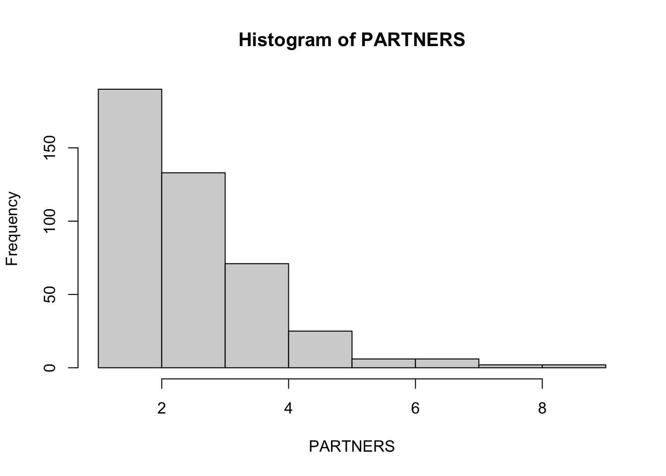
The distribution of PARTNERS is severely non-normal. Instead of attempting to transform the variable we will produce summary statistics for each level of the HIV variable and perform a non-parametric test:
by(PARTNERS, HIV, summary)
kruskal.test(PARTNERS ~ HIV)
## HIV: 0
## Min. 1st Qu. Median Mean 3rd Qu. Max.
## 1.00 2.00 3.00 2.72 3.00 8.00
## ------------------------------------------------------------
## HIV: 1
## Min. 1st Qu. Median Mean 3rd Qu. Max.
## 1.000 4.000 5.000 5.381 7.000 9.000##
## Kruskal-Wallis rank sum test
##
## data: PARTNERS by HIV
## Kruskal-Wallis chi-squared = 32.036, df = 1, p-value = 1.514e-08An alternative way of looking at the data is as a tabulation:
table(PARTNERS, HIV)## HIV
## PARTNERS 0 1
## 1 60 1
## 2 128 1
## 3 131 2
## 4 68 3
## 5 21 4
## 6 3 3
## 7 2 4
## 8 1 1
## 9 0 2
You can use the plot() function to represent this table graphically:
plot(table(PARTNERS, HIV), color = c("lightgreen", "red"))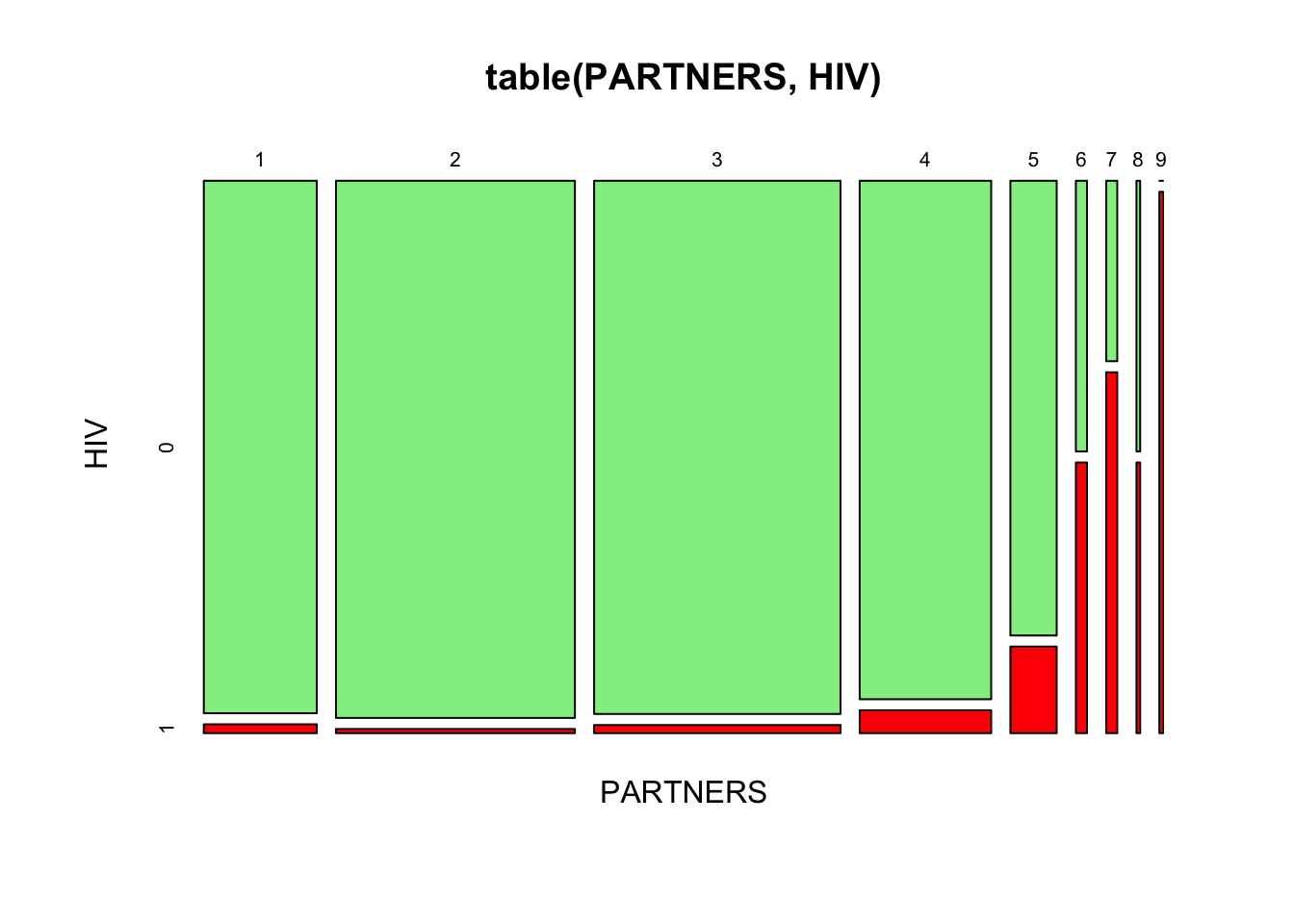
There appears to be an association between the number of sexual PARTNERS in the previous twelve months and positive HIV serology. The proportion with positive HIV serology increases as the number of sexual partners increases:
prop.table(table(PARTNERS, HIV), 1) * 100## HIV
## PARTNERS 0 1
## 1 98.3606557 1.6393443
## 2 99.2248062 0.7751938
## 3 98.4962406 1.5037594
## 4 95.7746479 4.2253521
## 5 84.0000000 16.0000000
## 6 50.0000000 50.0000000
## 7 33.3333333 66.6666667
## 8 50.0000000 50.0000000
## 9 0.0000000 100.0000000
The ‘1’ instructs the prop.table() function to calculate row proportions. You can also use the plot() function to represent this table graphically:
plot(prop.table(table(PARTNERS, HIV), 1) * 100, color = c("lightgreen", "red"))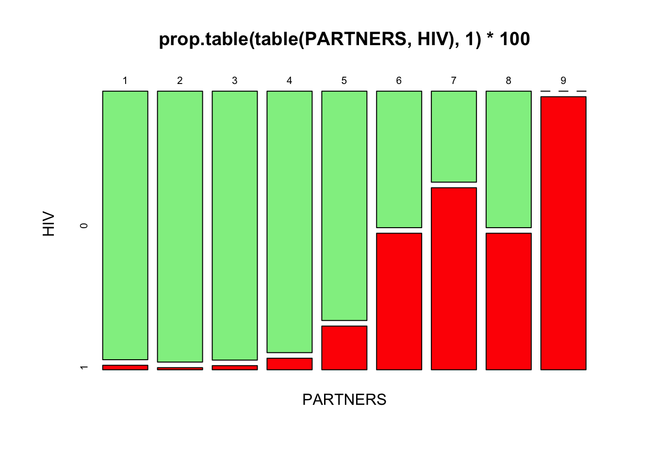
The chi-square test for trend is an appropriate test to perform on this data. The prop.trend.test() function that performs the chi-square test for trend requires you to specify the number of events and the number of trials. In this table:
table(PARTNERS, HIV)## HIV
## PARTNERS 0 1
## 1 60 1
## 2 128 1
## 3 131 2
## 4 68 3
## 5 21 4
## 6 3 3
## 7 2 4
## 8 1 1
## 9 0 2
The number of events in each row is in the second column (labelled 1) and the number of trials is the total number of cases in each row of the table.
We can extract this data from a table object:
tab <- table(PARTNERS, HIV)
events <- tab[ ,2]
trials <- tab[ ,1] + tab[ ,2]
tab <- table(PARTNERS, HIV)
events <- tab[ ,2]
trials <- tab[ ,1] + tab[ ,2]
Another way of creating the trials object would be to use the apply() function to sum the rows of the tab object:
trials <- apply(tab, 1, sum)Pass this data to the prop.trend.test() function:
prop.trend.test(events, trials)##
## Chi-squared Test for Trend in Proportions
##
## data: events out of trials ,
## using scores: 1 2 3 4 5 6 7 8 9
## X-squared = 76.389, df = 1, p-value < 2.2e-16
With a linear trend such as this we can use PARTNERS in a logistic model without recoding or creating indicator variables. We can now specify and fit the logistic regression model:
gudhiv.lreg <- glm(formula = HIV ~ GUD + TRAVOUT + PARTNERS,
                   family = binomial(logit))
summary(gudhiv.lreg)
##
## Call:
## glm(formula = HIV ~ GUD + TRAVOUT + PARTNERS, family = binomial(logit))
##
## Deviance Residuals:
## Min 1Q Median 3Q Max
## -1.70415 -0.19849 -0.11148 -0.06247 3.11742
##
## Coefficients:
## Estimate Std. Error z value Pr(>|z|)
## (Intercept) -9.4854 1.4663 -6.469 9.86e-11 ***
## GUD 1.3869 0.5937 2.336 0.0195 *
## TRAVOUT 2.0867 0.9547 2.186 0.0288 *
## PARTNERS 1.1605 0.2050 5.662 1.50e-08 ***
## ---
## Signif. codes: 0 '***' 0.001 '**' 0.01 '*' 0.05 '.' 0.1 ' ' 1
##
## (Dispersion parameter for binomial family taken to be 1)
##
## Null deviance: 167.364 on 425 degrees of freedom
## Residual deviance: 99.377 on 422 degrees of freedom
## (9 observations deleted due to missingness)
## AIC: 107.38
##
## Number of Fisher Scoring iterations: 8
We can use the lreg.or() function that we wrote earlier to calculate and display odds ratios and confidence intervals:
lreg.or(gudhiv.lreg)## OR LCI UCI
## (Intercept) 0.00 0.00 0.00
## GUD 4.00 1.25 12.81
## TRAVOUT 8.06 1.24 52.35
## PARTNERS 3.19 2.14 4.77
PARTNERS is incorporated into the logistic model as a continuous variable.
The odds ratio reported for PARTNERS is the odds ratio associated with a unit increase in the number of sexual PARTNERS. A man reporting five sexual partners, for example, was over three times as likely (odds ratio = 3.19) to have a positive HIV-2 serology than a man reporting four sexual partners.
An alternative approach would be to have created an indicator variables:
part.gt.5 <- ifelse(PARTNERS > 5, 1, 0)
This creates a new variable (part.gt.5) that indicates whether or not an individual subject reported having more than five sexual partners in the previous twelve months:
table(PARTNERS, part.gt.5)## part.gt.5
## PARTNERS 0 1
## 1 61 0
## 2 129 0
## 3 133 0
## 4 71 0
## 5 25 0
## 6 0 6
## 7 0 6
## 8 0 2
## 9 0 2
You can also inspect this on a case-by-case basis:
cbind(PARTNERS, part.gt.5)## PARTNERS part.gt.5
## [1,] 2 0
## [2,] 2 0
## [3,] 1 0
## [4,] 2 0
## [5,] 3 0
## [6,] 2 0
We can now specify and fit the logistic regression model using our indicator variable:
gudhiv.lreg <- glm(formula = HIV ~ GUD + TRAVOUT + part.gt.5,
                   family = binomial(logit))
summary(gudhiv.lreg)
lreg.or(gudhiv.lreg)
##
## Call:
## glm(formula = HIV ~ GUD + TRAVOUT + part.gt.5, family = binomial(logit))
##
## Deviance Residuals:
## Min 1Q Median 3Q Max
## -1.6092 -0.2205 -0.2205 -0.0719 3.4521
##
## Coefficients:
## Estimate Std. Error z value Pr(>|z|)
## (Intercept) -5.9559 0.9850 -6.046 1.48e-09 ***
## GUD 1.4930 0.5805 2.572 0.0101 *
## TRAVOUT 2.2514 0.9319 2.416 0.0157 *
## part.gt.5 4.6791 0.7560 6.189 6.05e-10 ***
## ---
## Signif. codes: 0 '***' 0.001 '**' 0.01 '*' 0.05 '.' 0.1 ' ' 1
##
## (Dispersion parameter for binomial family taken to be 1)
##
## Null deviance: 167.36 on 425 degrees of freedom
## Residual deviance: 106.43 on 422 degrees of freedom
## (9 observations deleted due to missingness)
## AIC: 114.43
##
## Number of Fisher Scoring iterations: 7## OR LCI UCI
## (Intercept) 0.00 0.00 0.02
## GUD 4.45 1.43 13.89
## TRAVOUT 9.50 1.53 59.02
## part.gt.5 107.67 24.47 473.84
We can now quit R:
q()
For this exercise there is no need to save the workspace image so click the No or Don’t Save button (GUI) or enter n when prompted to save the workspace image (terminal).
4.1 Summary
Using built-in functions and our own functions we can use
Rto analyse epidemiological data.The power of
Ris that it can be easily extended. Many user-contributed functions (usually packages of related functions) are available for download over the Internet. We will use one of these packages in the next exercise.